TensorFlow

Installation

Arguably the safest way to install TensorFlow is to use a self-contained virtual environment for the TensorFlow Python package and its dependencies. This method isolates the TensorFlow install from the operating system's Python environment and can help to mitigate broad, system-wide errors. A virtual environment 'tf_env' can be created in the directory '~/tf_folder' with the base python executable '/usr/bin/python3.n' as follows:

$ pip install virtualenv
$ cd tf_folder
$ virtualenv -p /usr/bin/python3.n tf_env

This virtual environment can then be invoked by running 'source ~/tf_folder/bin/activate'. For convenience, an alias such as 'tf' can be setup by adding the following to the '~/.bash_aliases' file in the home directory:

alias tf='source ~/tf_folder/bin/activate'

After entering the virtual environment, the TensorFlow library can be installed using the pip package manager:

(tf) $ pip3 install --upgrade [tfBinaryURL for Python 3.n]

The tfBinaryURLs are listed here. Additional details and installation options (e.g. for installing CUDA for GPU support) can be found at the TensorFlow page documentation page.

To leave/deactivate the virtual environment, run:

(tf) $ deactivate

and to completely remove the virtual environment simply remove the ~/tf_folder directory.

The TensorFlow library and associated data visualization package TensorBoard are also both included in the official Arch Linux repositories. These packages can be installed using the pacman package manager by running:

$ sudo pacman -S tensorflow tensorboard

Graphs and Sessions

TensorFlow uses the concept of a graph to define and store neural network models. The graph is defined by specifying a collection of placeholders, variables, and operations which map out all of the data structures and calculations that determinine the desired model. For example, a very simple graph can be constructed using the following code:

This defines all of the necessary data structures and operations required to add \(10.0\) to each entry of a vector \(x\) with unspecified length (since the shape of \(x\) is set to [None]). No operations are actually carried out in the code above, however; in order to execute an operations we must initialize a TensorFlow session and run the tf.add operation to execute the code:

In particular, we must first specify the actual values which should be used for the placeholder \(x\). Placeholders, as their name suggests, are used to mark the places where a given value will be used throughout the computational graph. The values of these placeholders are specified by 'feeding' in values using a feed dictionary, e.g. feed_dict={x:[1.,2.,3.]}.

Another common data structure in TensorFlow model is tf.Variable. Variables denote tensors whose values are permitted to change during the execution of the operations in the graph. In most cases, these data structures are used to store values which are intended to be changed (e.g. optimized) by operations within the TensorFlow graph.

The variable initializer tf.truncated_normal_initializer() plays a similar role to the feed dictionary for placeholders. The values of variables will be stored and modified by the graph operations throughout the training process, but we must first specify a value for each variable to start with. Initial values may be specified explicitly, but in most cases it is advisable to use some form of random initialization such as the one used in the example above.

Note: In addition to specifying the initializer to use, we must also actually execute this initialization; this is carried out by the init = tf.global_variables_initializer() and sess.run(init) lines.

It is also worth noting that we did not need to specify a feed dictionary to retrieve the slope and intercept values at the end of the training process. This does not raise an error because the values of these variables do not depend on the values of either of the placeholders.

Introductory Example

While there are a number of performance advantages motivating TensorFlow's graph-based evaluation strategy, it also entails a rather unintuitive coding style which may be difficult to get used to at first. The key idea to keep in mind is that the graph must first be defined (including e.g. loss functions, optimization procedures, and variable initializers) and then be evaluated (or run) in order for the graph operations to actually be executed. A very simple example of a fully-connected neural network trained to model the standard sine function \(\operatorname{sin}(x)\) on the interval \([-\pi/2, \pi/2]\) can be implemented as follows:

Here we have constructed a simple fully-connected network with three hidden layers, each using the rectified linear unit (ReLU) activation function tf.nn.relu. It is often important to remember to omit the activation function on the last layer of the network (by setting activation=None). In particular, the training process will fail quite miserably if the ReLU activation function is used for the final prediction since all predictions will be non-negative.

There are situations where a specific activation function may be well-suited for making the final prediction, however; for example, if we are interested in predicting a probability it is often convenient to use the sigmoidal activation function tf.nn.sigmoid in order to ensure all predictions are made in the interval \([0,1]\).

The training process for this simple model should take only a few seconds (so we have omitted providing feedback regarding the training status) and produces a fairly accurate approximation to the true sine function:

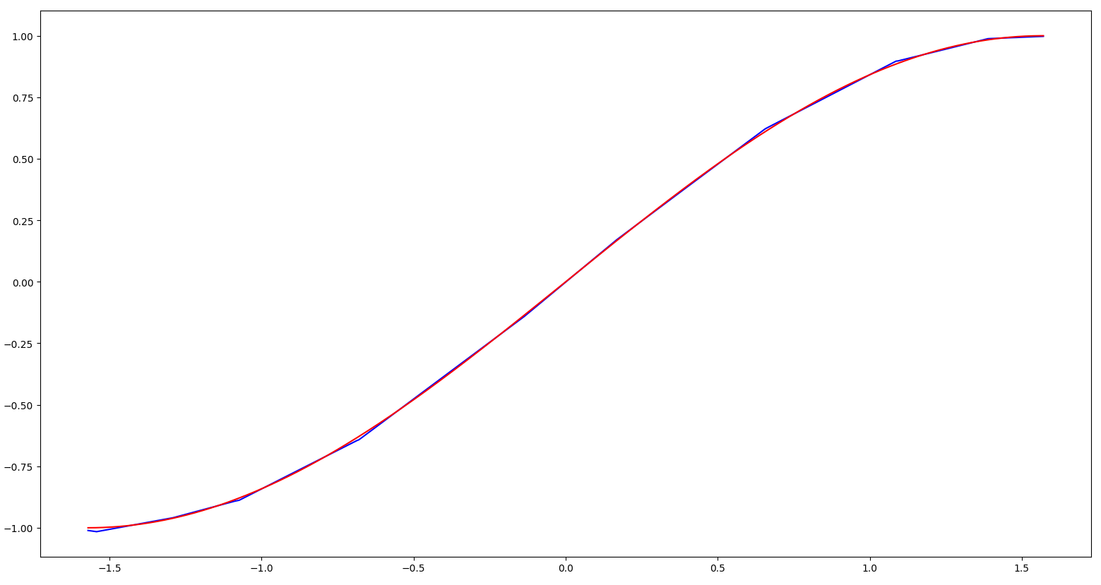
Predicted values are shown in blue; true values of the sine function are shown in red.

Lorem ipsum dolor sit amet, consectetur adipisicing elit, sed do eiusmod tempor incididunt ut labore et dolore magna aliqua. Ut enim ad minim veniam, quis nostrud exercitation ullamco laboris nisi ut aliquip ex ea commodo consequat. Lorem ipsum dolor sit amet, consectetur adipisicing elit, sed do eiusmod tempor incididunt ut labore et dolore magna aliqua. Ut enim ad minim veniam, quis nostrud exercitation ullamco laboris nisi ut aliquip ex ea commodo consequat.

Network Layers

As shown in the previous example, TensorFlow offers predefined network layers in the tf.layers module. These layers help streamline the process of variable creation and initialization for many of the most commonly used network layers . In addition, these layers offer a way to easily specify the use of activation functions, bias terms, and regularization.

Some of the most frequently network layers which are included in the tf.layers module are listed below:

• tf.layers.dense
• tf.layers.conv2d
• tf.layers.conv2d_transpose
• tf.layers.dropout
• tf.layers.max_pooling2d
• tf.layers.average_pooling2d
• tf.layers.batch_normalization

The full list of predefined network layers available, along with descriptions of the associated options, can be found on the official TensorFlow Python API documentation page.

Loading Data

In the previous examples, artificial data has been created 'on-the-fly' during the training process. In practice, we typically have an existing, fixed dataset that will be used to train the model. The process of loading, shuffling, and grouping data into mini-batches can be carried out using the tf.data.Dataset submodule. When the dataset is stored in numpy arrays we can use the tf.data.Dataset.from_tensor_slices constructor to define a data loader as follows:

Here the data loader is instructed to 'prefetch' five mini-batches at a time and also shuffles and repeats the dataset after each epoch. In particular, we can train for \(20000\) steps to make two full passes through the full dataset (i.e. train for two epochs).

Note: When training for multiple epochs it is advisable to decrease the learning rate as the training process progresses. As shown above, this can be accomplished by using a placeholder to define the learning rate in the graph and feeding in a value which decays after a specified number of steps.

Caution: In most cases, the learning rate should not be adjusted within an epoch since this will bias the learning process toward modelling the early samples more accurately than the later samples; the simple implementation for this example has been chosen for pedagogical purposes.