Deep Learning

Feedforward Networks

The fundamental building block of feedforward neural networks is the fully-connected neuron illustrated below:

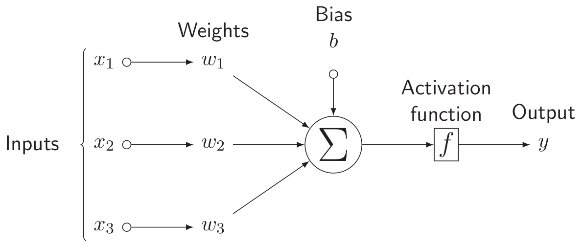
Diagram modified from Stack Exchange post answered by Gonzalo Medina.

In particular, the output is defined by the formula \[ y \, = \, f\left(\sum\nolimits_j w_{j} \, x_j \, + \, b \right) \] where \(w_{j}\) denote the network weights, \(\,b\) denotes a bias term, and \(f\) denotes a specified activation function. A natural extension of this simple model is attained by combining multiple neurons to form a so-called hidden layer:

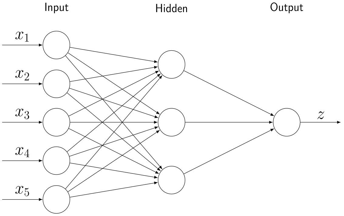
Diagram modified from Stack Exchange post answered by Gonzalo Medina.

The hidden layer values are then given by: \[ y_i \, = \, f\left(\sum\nolimits_j w_{i,j} \, x_j \, + \, b_i \right) \] and the final output is given by: \[ z \, = \, f\left(\sum\nolimits_k w^{(z)}_{k} \, y_k \, + \, b^{(z)} \right) \]

Using matrix notation this can be expressed more concisely via: \[ {\bf{y}} \, \, = \, \, f\left( W \, {\bf{x}} \, + \, {\bf{b}}\right)\] \[ z \, \, = \, \, f\left( W^{(z)} \, {\bf{y}} \, + \, b^{(z)} \right) \]

More generally, we can construct a network architecture with multiple hidden layers and a multi-dimensional output:

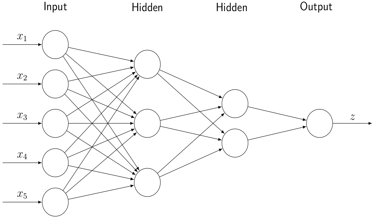
In this case we can again express the underlying mathematical equations concisely using matrix notation: \[ {\bf{y}}^{(1)} \, \, = \, \, f\left( W^{(1)} \, {\bf{x}} \, + \, {\bf{b}}^{(1)}\right) \] \[ {\bf{y}}^{(2)} \, \, = \, \, f\left(W^{(2)} \, {\bf{y}}^{(1)} \, + \, {\bf{b}}^{(2)}\right)\] \[ {\bf{z}} \, \, = \, \, f\left(W^{(z)} \, {\bf{y}}^{(2)} \, + \, {\bf{b}}^{(z)}\right) \]

The above fully-connected network model generalizes naturally to an arbitrary number of hidden layers. For comparison with alternative network architectures, we note the connection between a layer with \(N\) nodes and a layer with \(M\) nodes entails:

\[ \begin{array}{|c|c|} \hline \hspace{0.25in} \mbox{FLOPs} \hspace{0.25in} & \hspace{0.25in} \mbox{Weights} \hspace{0.25in} \\ \hline 2 \, M \, N & M\, N \\ \hline \end{array} \]

The floating point operation (FLOP) count consists of the \(M\) addition operations for including the bias terms along with the \(M\cdot N\) multiplication operations and \(M\cdot(N-1)\) addition operations required for matrix-vector multiplication of the weight matrix with the input/previous-layer values.

A good introductory reference for counting floating point operations can be found at the following link:

• Floating Point Operations in Matrix-Vector Calculus (Raphael Hunger, 2007)

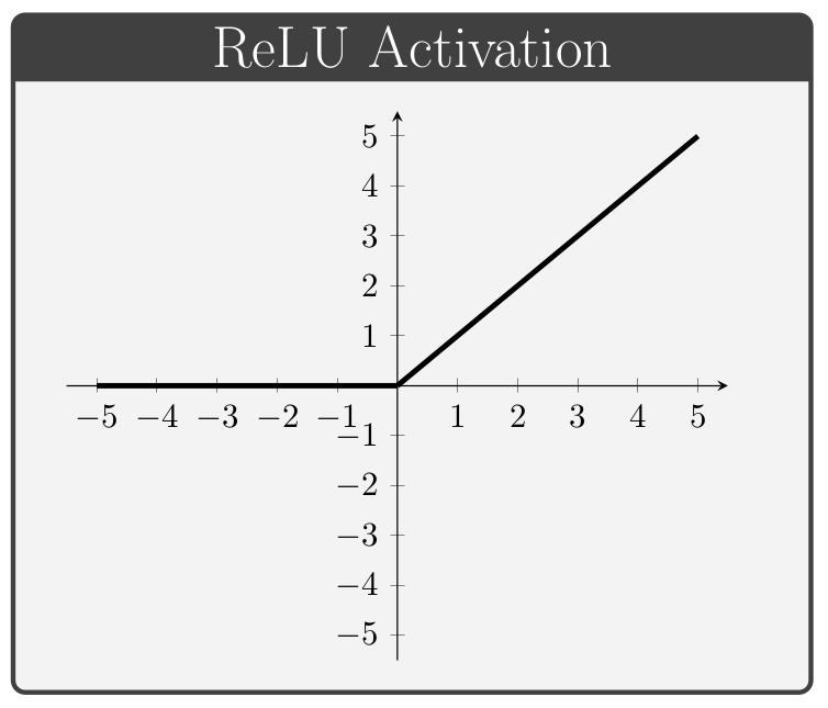
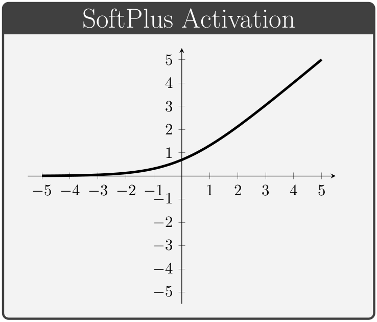
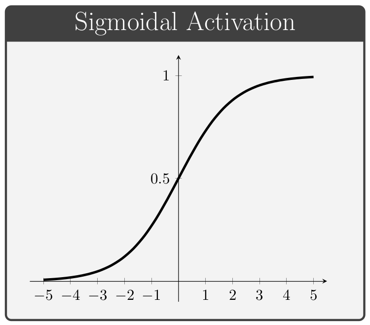
Activation Functions

The activation function, denoted by \(\,f\) above, is a key component of neural network architectures. These functions provide all of the network's non-linear modeling capacity and are responsible for controlling the gradient flows which guide the training process. In this section we briefly review a collection of common activation functions; of note is the fact that different activation functions can be used for different layers within a given network.

Rectified Linear Unit (ReLU) \[ f(x) \, \, = \, \, \begin{cases} \, \, x & \, \, x \geq 0 \\ \, \, 0 & \, \, x < 0\end{cases}\]	SoftPlus Activation \[ f(x) \, \, = \, \, \ln\big(1 \, + \, \exp(x)\big) \]
Sigmoidal Unit \[ f(x) \, \, = \, \, \frac{1}{1 \, + \, \exp(-x)} \]	Hyperbolic Tangent Unit \[ f(x) \, \, = \, \, \operatorname{tanh}(x) \]
Exponential Linear Unit (ELU) \[ f_{\alpha}(x) \, \, = \, \, \begin{cases} \, \, x & \, \, x \geq 0 \\ \, \, \alpha\cdot (e^x \, - \, 1) & \, \, x < 0\end{cases}\]	Leaky Rectified Linear Unit (Leaky ReLU) \[ f_{\alpha}(x) \, \, = \, \, \begin{cases} \, \, x & \, \, x \geq 0 \\ \, \, \alpha\cdot x & \, \, x < 0\end{cases}\]
Parameterized Rectified Linear Unit (PReLU) \[ f_{\beta}(x) \, \, = \, \, \begin{cases} \, \, \beta\cdot x & \, \, x \geq 0 \\ \, \, x & \, \, x < 0\end{cases}\]	Swish Units \[ f_{\beta}(x) \, \, = \, \, \frac{x}{1 \, + \, \exp(-\beta\cdot x)} \]

Rectified Linear Unit (ReLU) \[ f(x) \, \, = \, \, \begin{cases} \, \, x & \, \, x \geq 0 \\ \, \, 0 & \, \, x < 0\end{cases}\]

SoftPlus Activation \[ f(x) \, \, = \, \, \ln\big(1 \, + \, \exp(-x)\big) \]

Sigmoidal Unit \[ f(x) \, \, = \, \, \frac{1}{1 \, + \, \exp(-x)} \]

Hyperbolic Tangent Unit \[ f(x) \, \, = \, \, \operatorname{tanh}(x) \]

Exponential Linear Unit (ELU) \[ f_{\alpha}(x) \, \, = \, \, \begin{cases} \, \, x & \, \, x \geq 0 \\ \, \, \alpha\cdot (\exp(x) \, - \, 1) & \, \, x < 0\end{cases}\]

Leaky Rectified Linear Unit (Leaky ReLU) \[ f_{\alpha}(x) \, \, = \, \, \begin{cases} \, \, x & \, \, x \geq 0 \\ \, \, \alpha\cdot x & \, \, x < 0\end{cases}\]

Parameterized Rectified Linear Unit (PReLU) \[ f_{\beta}(x) \, \, = \, \, \begin{cases} \, \, \beta\cdot x & \, \, x \geq 0 \\ \, \, x & \, \, x < 0\end{cases}\]

Swish Units \[ f_{\beta}(x) \, \, = \, \, \frac{x}{1 \, + \, \exp(-\beta\cdot x)} \]

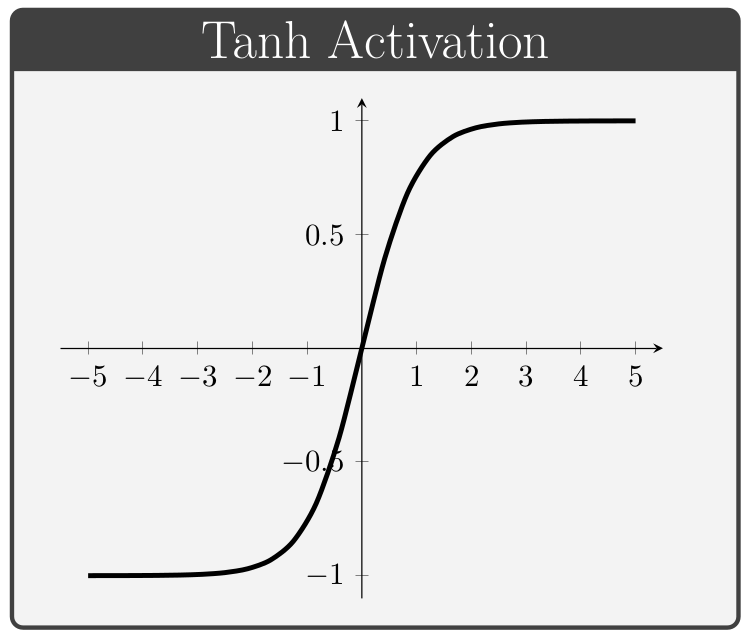
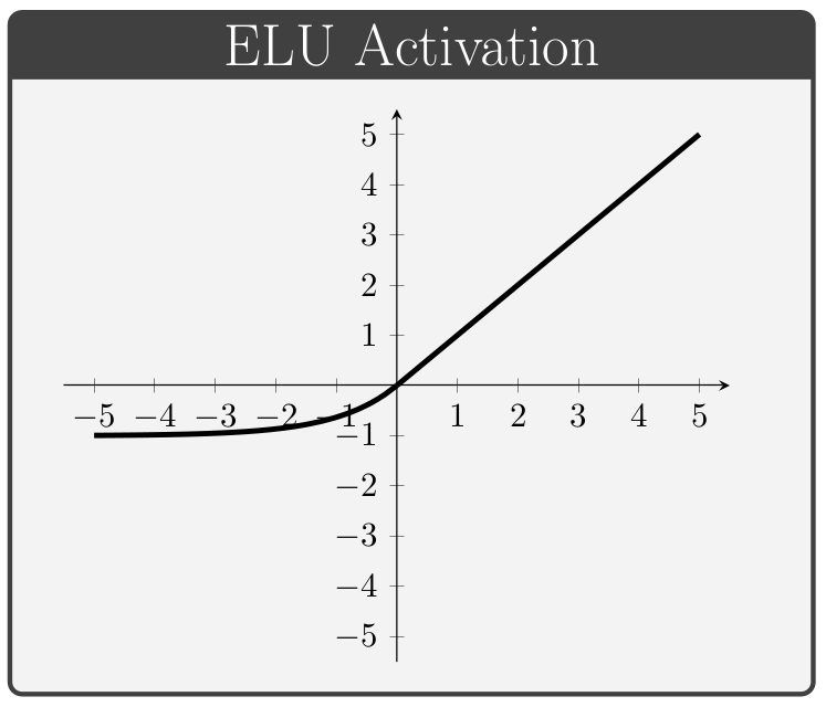
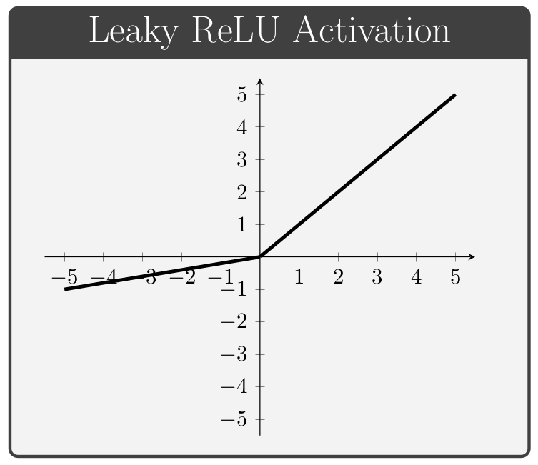
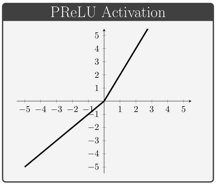
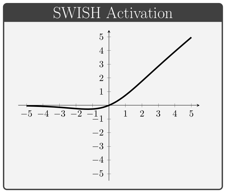
Conventionally, the values of \(\alpha\) in the ELUs and Leaky ReLUs are treated as hyper-parameters (i.e. values specified manually prior to training) whereas the values of \(\beta\) in the PReLUs and Swish units are taken to be trainable variables (i.e. values which the network is permitted to change during the learning process).

Convolutional Layers

In many cases the spatial orientation of the input data plays an important role in the correct interpretation of the data. Fully-connected layers are extremely inefficient at learning spatial connections, however, since the ordering/arrangement of the data has no influence in the overall network architecture (in the sense that if all entries of the input dataset were permuted in a fixed manner, the performance of the network would remain unchanged).

Convolutional layers are specifically suited for processing data with spatial features (e.g. images, time-series, etc.). The fundamental idea behind convolutional layers is to restrict the domain of influence of any given input; in particular, convolutional layers specify a receptive field which determines which ouput neurons are affected by each input value.

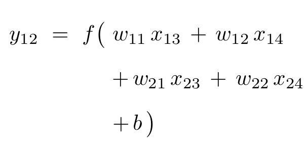
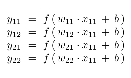
A typical example of a convolutional layer consists of a \(2\times2\) filter with stride \(2\). The filter size determines how many distinct input values will be used to compute a given output value. This filter is illustrated as a gray square in the diagram below.

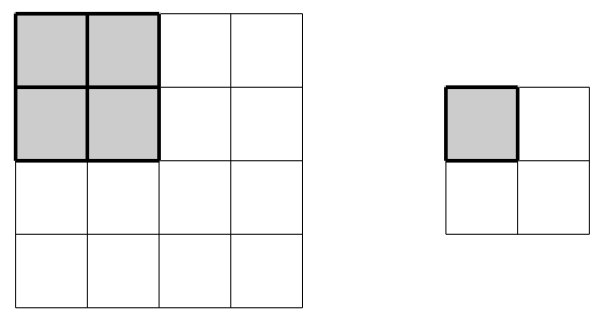
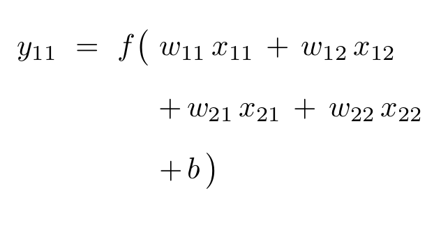
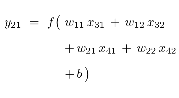
The filter is designed to slide across the input array to produce output values by multiplying filter weights with the input values covered by the current filter position. The stride refers to the number of steps the filter slides after each calculation; in the example below the filter starts in the upper-left to produce the output value \(y_{11}\), shifts two steps right to align with the upper-right entries and produce the value \(y_{12}\), then shifts two steps down to repeat the process on the lower entries of the array.

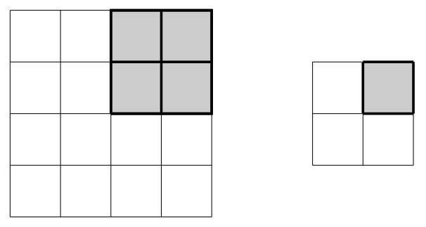
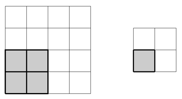
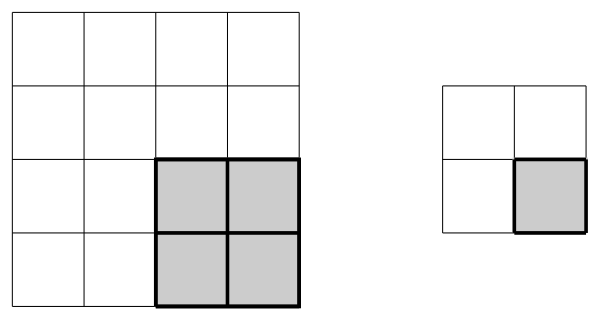
The process can be visualized as follows:

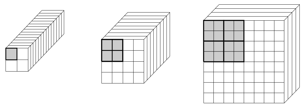
The use of a stride results in a reduction in the spatial dimension of the array. In order to maintain a sufficient amount of data in the output of a convolutional layer, it is standard to increase the number of channels (i.e. the number of distinct arrays produced) whenever the spatial resolution of an array is reduced. A typical example of a series of convolutional layers is illustrated below:

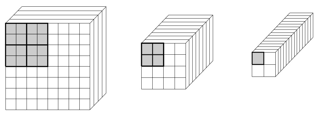
In the figure above, the receptive fields corresponding to the upper-left entries of the \(2\times2\) features on the right are marked with gray shading. For the \(4\times4\) features in the center, only the \(4\) entried in the upper-left-hand corner play a role in determining the value of the final upper-left entries in the \(2\times2\) features. As we move further back in the network, i.e. to the \(8\times8\) features on the left, we see that the receptive field has grown to \(16\) entries, each of which indirectly influences the final values taken by the upper-left entries in the \(2\times2\) features on the right.

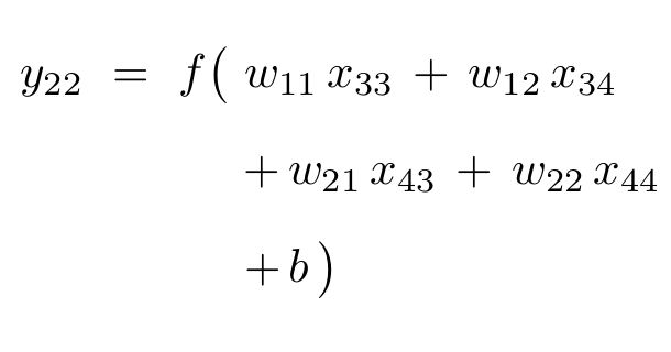
Up until now, we have only discussed convolutional layers between two arrays with a single channel; however, the concept generalizes naturally to multi-channel arrays. A convolutional layer between an input array with \(N\) channels and an ouput array with \(M\) channels is defined by a collection of \(N\cdot M\) distinct filters, with associated weight matrices \({\bf{W}}^{(n,m)}\) for \(\,n\in\{1,\dots,N\}\,\) and \(\,m\in\{1,\dots,M\}\,\), corresponding to the connections between each input channel and each output channel. In addition, each output channel is also assigned a bias term, \(\,b^{(m)}\in \mathbb{R}\,\) for \(m\in\{1,\dots,M\}\), and the final outputs for the \(m^{th}\) channel are given by: \[ {\bf{y}}^{(m)} \, \, = \, \, f\left( \, \sum\nolimits_n {\bf{W}}^{(n,m)}\, {\bf{x}}^{(n)} \, + \, b^{(m)} \, \right) \]

In some applications it is necessary to restore the original resolution of the input array. This requires an upsampling technique designed to increase the resolution of an array. It is often possible to upsample directly using a technique such as bilinear interpolation. The concept of convolutional layers also admits a natural generalization, however, which provides an alternative method for upsampling. For reasons that will be explained in the following section, the resulting layer is referred to as a transpose convolutional layer and is illustrated below:

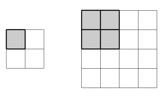
As we will see in the following section, almost all of the entries of the weight matrix \({\bf{W}}^T\) are zero (i.e. the matrix is extremely sparse). In particular, there is only one non-zero entry in each of the rows corresponding to the outputs \(\,y_{11}\), \(\,y_{12}\), \(\,y_{21}\), and \(\,y_{22}\); this non-zero entry corresponds to the input \(\,x_{11}\) which completely determines the entire upper-left corner of the output.

Similar to the case of convolutional layers, transpose layers should also be designed with the overall data size in mind. As the spatial resolution increases during the upsampling process, it is natural to reduce the number of channels to balance the total number of data entries:

For a more detailed explanation of convolutional layers, padding, and strides (i.e. convolutional arithmetic), please refer to the following GitHub repository and associated paper:

• Convolutional Arithmetic (Victor Dumoulin / vdumoulin)
• A Guide to Convolutional Arithmetic for Deep Learning (Dumoulin and Visin, 2016)

Another good reference can be found at the following link:

• Understanding Convolutional Layers

Matrix Representations

As mentioned in the discussion of fully connected layers, matrix representations offer a natural way of expressing the connection between network layers. Convolutional layers are also easily expressed in matrix form, however the dense weight matrices from fully-connected layers are replaced with highly structured, sparse matrices.

For example, the matrix representation for applying a convolutional layer with a \(2\times2\) filter and stride \(2\) to a \(4\times4\) input layer is given by:

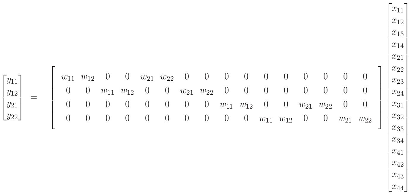
Note: Here we have omitted the activation function and bias terms for brevity. The key observation is that the \(y_{11}\) entry, for example, is only affected by the four upper-left input entries: \(\,x_{11}\), \(\,x_{12}\), \(\,x_{21}\), \(\,x_{22}\).

From the above matrix representation, we note that a stride \(1\), \(k\times k\) convolutional layer between a layer with resolution \(R\times R\) and \(N\) channels and a layer with \(M\) channels entails:

\[ \begin{array}{|c|c|} \hline \hspace{0.25in} \mbox{FLOPs} \hspace{0.25in} & \hspace{0.25in} \mbox{Weights} \hspace{0.25in} \\ \hline %\left(k^2\cdot(R \, - \, k)^2 \, + \, 1\right)\cdot N\cdot M & k^2 \cdot N\cdot M \\ \, \approx \, 2 \, k^2 \, R^2 \, N \, M \, & k^2 \, N\, M \\ \hline \end{array} \]

Here the FLOP calculation is carried out as follows: \[ k^2 \, R^2 \, N\, M \, + \, (k^2 - 1) \, R^2 \, N\, M \, + \, R^2\,(N-1)\, M \, + \, R^2 \, M \] \[ = \, \, 2 \, k^2 \, R^2 \, N\, M \] The first term corresponds to the multiplication operations with the filter weights in each filter position, the second term corresponds to the addition operations for each position, the third term accounts for the addition operations between the filtered input channels, and the last term accounts for the addition operations for including bias terms. This calculation is only approximate since it does not account for padding considerations (which will typically reduce the overall count by a negligible amount).

The transpose convolutional layer is defined, as the name suggests, by a weight matrix corresponding to the transpose of a standard convolutional weight matrix:

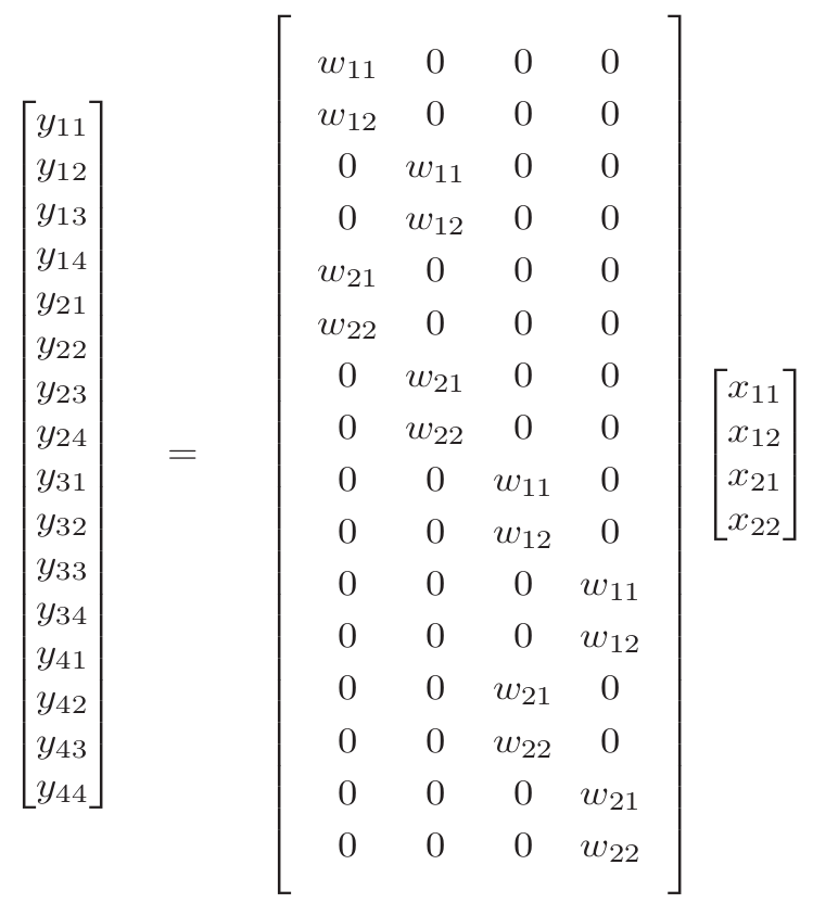
Note: Again, we have omitted the activation function and bias terms for brevity. The key observation is that the \(x_{11}\) entry, for example, is responsible for determining each of the four upper-left output entries: \(\,y_{11}\), \(\,y_{12}\), \(\,y_{21}\), \(\,y_{22}\).

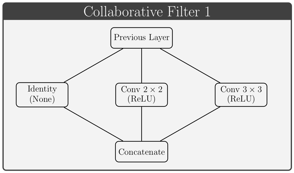
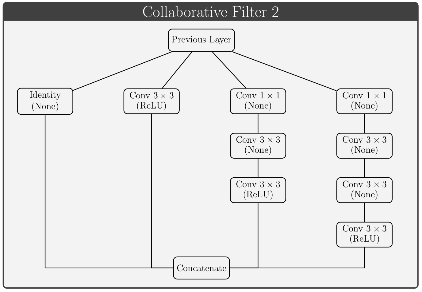
Collaborative Filters

Lorem ipsum dolor sit amet, consectetur adipisicing elit, sed do eiusmod tempor incididunt ut labore et dolore magna aliqua. Ut enim ad minim veniam, quis nostrud exercitation ullamco laboris nisi ut aliquip ex ea commodo consequat. Lorem ipsum dolor sit amet, consectetur adipisicing elit, sed do eiusmod tempor incididunt ut labore et dolore magna aliqua. Ut enim ad minim veniam, quis nostrud exercitation ullamco laboris nisi ut aliquip ex ea commodo consequat.